When property seekers view a listing on a real estate portal, they want to know what living there feels like: Would my daily commute work without a car? Are groceries and a pharmacy within walking distance? Is there a park or running route nearby?
Calculating location scores in real time for millions of map interactions would overwhelm traditional database architectures. Instead, Mapalizer precomputes spatial scores into discrete tiles, caches them as lightweight JSON files on a global CDN, and resolves client queries in milliseconds.
In this technical guide, we open the engine room. We trace the architecture from macro tiles to micro geometry: how the globe is sliced, how vector distances to real world geometries are measured, and how final scores are capped.
1. Slicing the Globe
Mapalizer divides geographical space into hierarchical indexed tiles across multiple zoom levels. At the base neighborhood level (zoom 14), each tile spans 0.1 degrees of longitude by 0.1 degrees of latitude.
To maintain fast visual rendering when users zoom out to wider regions, Mapalizer also precomputes parent layers:
- Zoom 14 (Street / Neighborhood): 0.1° layer size (approx. 11 km × 6.8 km in Berlin). Base scoring resolution.
- Zoom 12 (City District): 0.4° layer size.
- Zoom 10 (Metropolitan Area): 1.6° layer size.
- ...
Each tile is addressed by a coordinate path: {Z}/[e|w]/{X}/[n|s]/{Y}.json, representing zoom level, directional hemisphere, and grid index. For example, central Berlin at zoom 14 falls inside tile 14/e/134/n/525.json (spanning 13.4° to 13.5° East and 52.5° to 52.6° North).
2. Measuring OpenStreetMap Geometries
OpenStreetMap amenities are not just points on a map. Real world features possess three distinct geometric forms:
- Point: A single coordinate pair (for example, a cafe, bakery, or pharmacy).
- LineString: An ordered series of connected segments (for example, a bike path, running route, or river).
- Polygon: A closed boundary ring (for example, a city park, shopping center, or sports stadium).
For every grid point, Mapalizer computes the shortest distance to the feature boundary:
- To a Point: Flat Euclidean distance taking cosine scale into account.
- To a LineString: The perpendicular distance to the closest line segment, or to the nearest segment vertex if the perpendicular falls outside.
- To a Polygon: The minimum distance to the outer boundary ring. If a grid point falls inside the polygon, the distance is zero (yielding maximum contribution points).
3. The Evaluation on the Tile Grid Point
Now that we understand how the grid is structured and how distances are measured, let us examine how a single grid point becomes a category score.
Each Mapalizer category is divided into subcategories that represent different everyday needs. For this example, we examine the Dining category at a real Berlin grid point. Dining contains three subcategories: Restaurants, Cafes, and Bars & Pubs. Amenities compete only with others in the same subcategory, and the amenity with the strongest distance-based contribution becomes that subcategory's winner. This prevents several nearby venues serving the same need from being counted repeatedly.
Step A: Group Amenities by Need
Related OpenStreetMap tags are combined within each subcategory before its winner is selected.
Step B: Apply Linear Distance Decay
An amenity close by contributes far more than one further away. Each related OpenStreetMap tag is assigned its own rule, with a maximum contribution (m) and a cutoff distance (d). This means tags grouped within the same subcategory can use different m and d values. Between distance zero and distance d, score contribution drops linearly:
Could not load the example data for this section.
Step C: Select the Winner and Combine Subcategories
Within any subcategory, candidate amenities compete. The candidate amenity with the highest individual score wins, and its contribution is limited to the subcategory's maximum score. Additional candidates within this subcategory do not award extra points.
| Subcategory | Winning Amenity | Distance | Contribution | Theoretical Max |
|---|
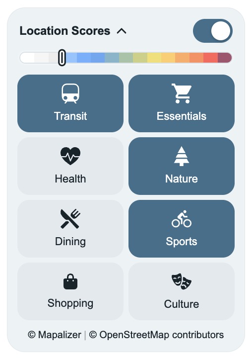
For every evaluation point in the tile grid, Mapalizer calculates total scores in the same way for all eight main categories: Transit, Essentials, Health, Nature, Dining, Sports, Shopping, and Culture. The production tile JSON object stores only these total category scores.
Up to this point, we have described how the score data is prepared. The following sections explain the processing performed on the client side in the browser.
4. From Categories to the Overall Mapalizer Score
5. Rendering Score Contours
How does Mapalizer convert a grid of discrete numeric scores into the smooth, organic colored contours rendered on interactive listing maps?
Instead of generating static raster image tiles, Mapalizer generates vector SVG polygons directly inside the user's web browser.
This client-side approach is essential: users can select any combination of the 8 categories. With 8 independent categories, there are 255 possible combinations (28 - 1 = 255). Generating vector contours client-side allows any custom combination to render dynamically and instantaneously.
layer.contourColors
Contour boundaries are computed with the Marching Squares algorithm via d3-contour, then each resulting ring is simplified with the Douglas-Peucker algorithm via simplify-js to keep the polygon lightweight. The simplified rings are drawn as native SVG <path> elements rendered directly by the browser.
Recap
Mapalizer turns precomputed tile grids into responsive location intelligence by measuring each grid point against real OpenStreetMap geometries, selecting the strongest amenity within each subcategory, and combining category scores through configurable weights. The result is compact data that can become smooth vector contours directly in the browser.